Create and Simulate¶

The definition of an ARMA model is:

$A(L)y_t = B(L)e_t + C(L)u_t$

where $L$ is the lag operator, $y_t$ a $p$ -dimensional vector of observed output variables, $e_t$ a $p$ -dimensional vector of white noise and $u_t$ a $m$ -dimensional vector of input variables. Since $A, B$ and $C$ are matrices in the lag shift operator, we have $A(L)$ is a $a \times\, p \times\, p$ tensor to define auto-regression, $B(L)$ is a $b \times\, p \times\, p$ tensor to moving-average and $C(L)$ is a $c \times\, p \times\, m$ tensor to account for the input variables.

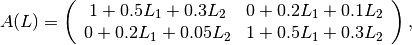
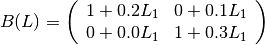
We create a simple ARMA model for a two dimensional output vector with matrices:

$A(L) = \left( \begin{array}{cc} 1+0.5L_1+0.3L_2 & 0+0.2L_1+0.1L_2\\ 0+0.2L_1+0.05L_2 & 1+0.5L_1+0.3L_2\end{array} \right),$

$B(L) =\left( \begin{array}{cc} 1+0.2L_1 & 0+0.1L_1\\ 0+0.0L_1 & 1+0.3L_1\end{array} \right)$

In order to set this matrix we just write the entries left to right, up to down into an array and define the shape of this array in a second array:

import pandas as pd
import numpy as np
import matplotlib.pylab as plt
from pydse.arma import ARMA

AR = (np.array([1, .5, .3, 0, .2, .1, 0, .2, .05, 1, .5, .3]), np.array([3, 2, 2]))
MA = (np.array([1, .2, 0, .1, 0, 0, 1, .3]), np.array([2, 2, 2]))
arma = ARMA(A=AR, B=MA, rand_state=0)

(Source code)

Note that we set the random state to seed 0 to get the same results. Then by simulating we get:

sim_data = arma.simulate(sampleT=100)
sim_index = pd.date_range('1/1/2011', periods=sim_data.shape[0], freq='d')
df = pd.DataFrame(data=sim_data, index=sim_index)
df.plot()

(Source code, png, hires.png, pdf)

(Source code)

Let’s create a simpler ARMA model with scalar output variable.

AR = (np.array([1, .5, .3]), np.array([3, 1, 1]))
MA = (np.array([1, .2]), np.array([2, 1, 1]))
arma = ARMA(A=AR, B=MA, rand_state=0)

(Source code)

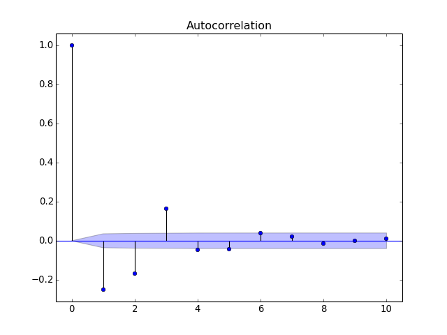
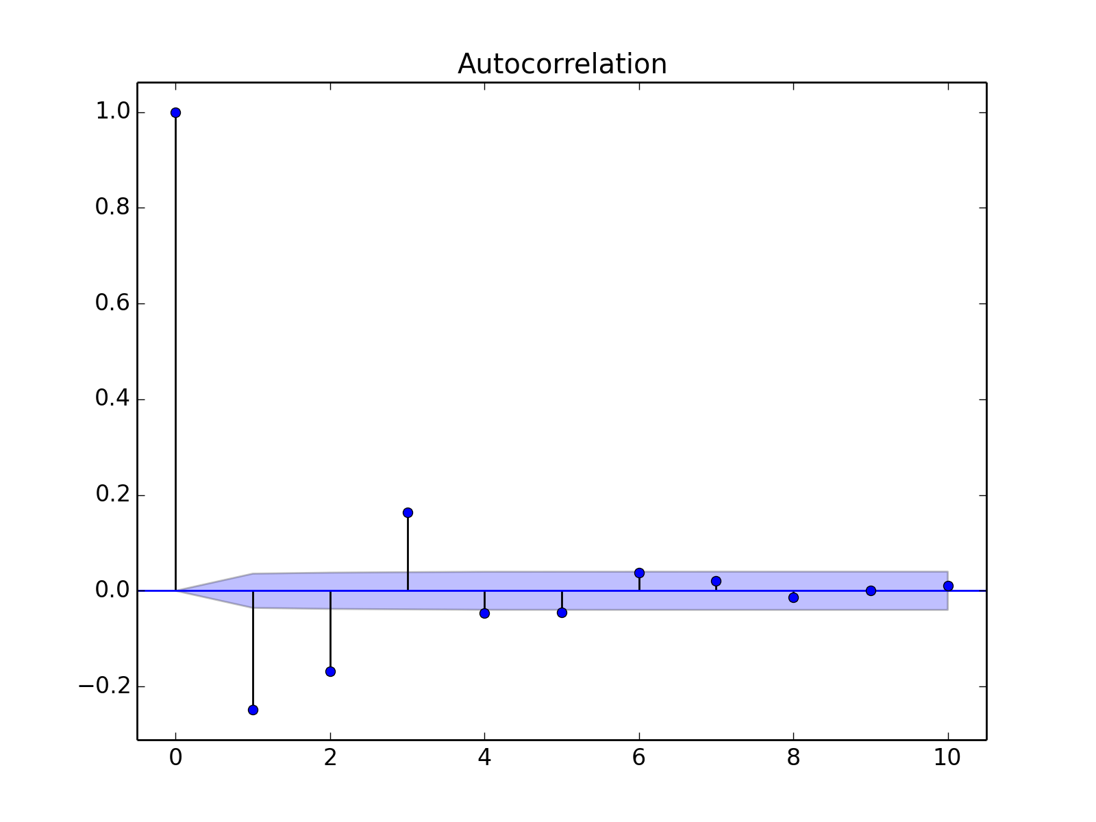
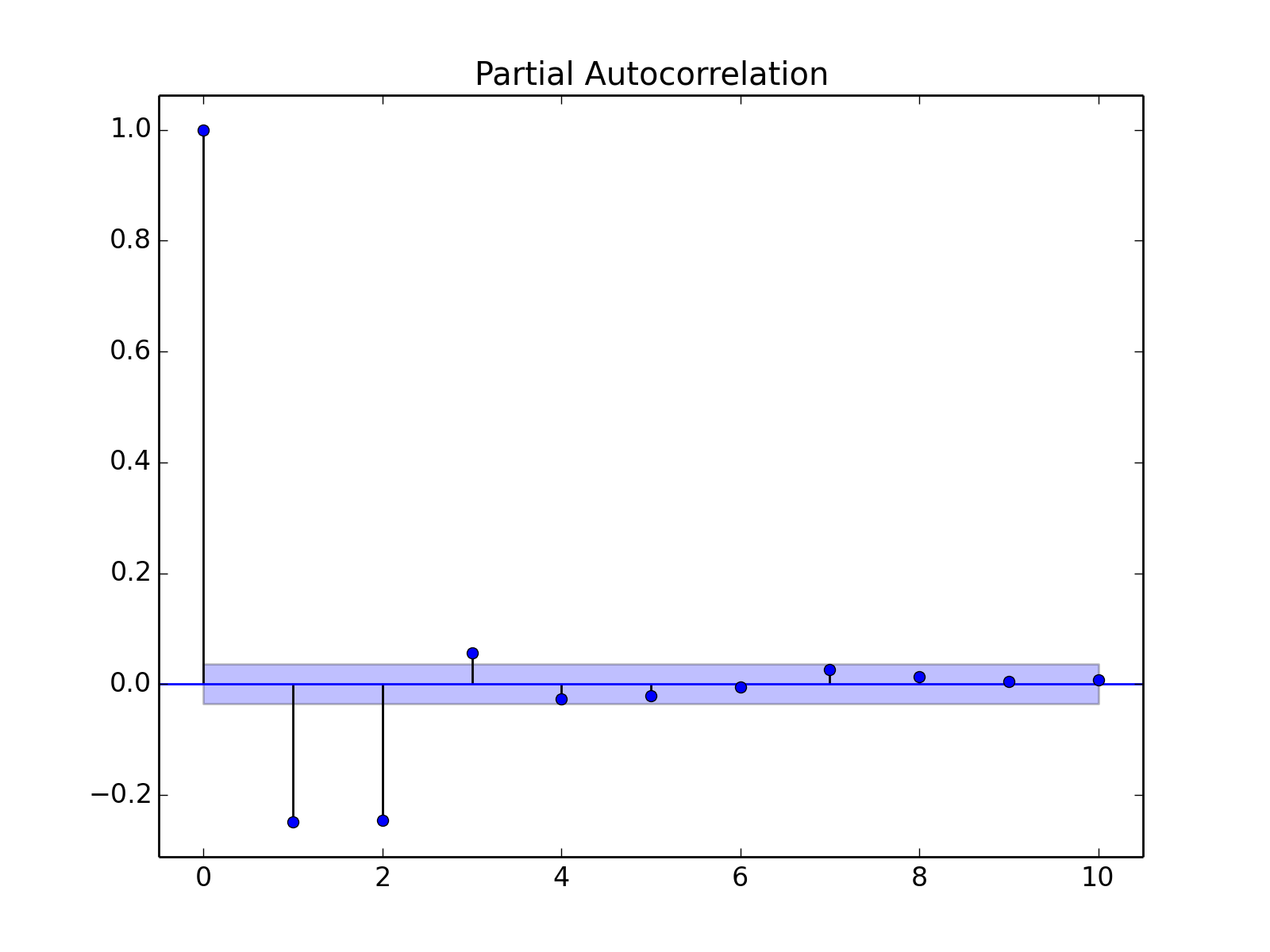
Quite often you wanna check the autocorrelation function and partial autocorrelation function:

from statsmodels.graphics.tsaplots import plot_pacf, plot_acf

sim_data = arma.simulate(sampleT=3000)
sim_index = pd.date_range('1/1/2011', periods=sim_data.shape[0], freq='d')
df = pd.DataFrame(data=sim_data, index=sim_index)
plot_acf(df[0], lags=10)
plot_pacf(df[0], lags=10)
plt.show()

(Source code)

(png, hires.png, pdf)

(png, hires.png, pdf)

Find a good introduction to ARMA on the Decision 411 course page.